How to heatmap data with conditional formatting colour scales (row by row)

If you have ever worked with the advanced conditional formatting you'll know it can be a bit of a challenge, especially if you in a rush and all you want to is finish your excelling so you can actually analyse your data! In the data-driven world of analytics, we work with boatloads of data each day and sometimes analysing these trends in quick and obvious ways can be less tedious than you think.

One of my favourite tricks is applying a heat map to a range of data by row so you can analyse when each variable performs at its best - like this: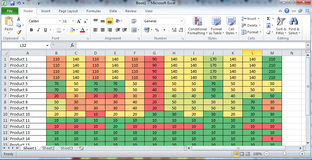

This can easily be done using the conditional formatting colour-scales feature for a single row. The problem comes in when your data set is hundreds of variables long and applying this method to all of them will take you a better part of the day (hours of your life which you will never get back!) which can be used more constructively! The good news is that as always, I have a trick up my sleeve! Here are two much more efficient ways to apply colour scales to your data to each row independently.

Copy and Paste

Yes, the answer is as simple as copy and paste. The easiest way to achieve this is to:

• First format the first row using the colour scales gradient you prefer, I usually choose the Green - Yellow - Red gradient.
• Highlight the first row and copy
• Highlight the second row and past special, values only.
• Now copy both rows and paste special to rows 3 and 4.
• Now copy 4 and paste 4, and continue like this until all cells have been covered.

While this is the easiest way, it's still not the fastest way if you working with a large dataset.

Using Macros

The good news is if you familiar with macros there is an easier way. The macro below will copy the conditional formatting you applied to the first row of data and apply it to each row you select (independently).

Just REPLACE B1: M1 and reference the first row of your table.

Sub nicheCF()
Range("B1:P1").Copy
For Each r In Selection.Rows
r.PasteSpecial (xlPasteFormats)
Next r
Application.CutCopyMode = False
End Sub

How to use:

• Apply the formatting to the first row.
• Highlight all the unformatted rows (only the cells you want to format)
• Run the macro
• Sit back and enjoy your coffee while the magic happens!

The bulk formatting usually goes quite fast, but the time it takes is directly dependant on the size of the dataset.

That's it! You're done!

Contact us

If you have any questions or would like to know more about conditional formatting, comment below or feel free to contact us here!

Tags: conditional formatting, Data Analysis, excel, How to